Visualizing physical quantities for regular 3-d grids#
As described in Extracting physical quantities, it is easy to extract quantities such as density, specific_energy, and temperature from the output model files. In this tutorial, we see how to visualize this information efficiently.
Cartesian grid example#
We first set up a model of a box containing 100 sources heating up dust:
import random
random.seed('hyperion')  # ensure that random numbers are the same every time

import numpy as np
from hyperion.model import Model
from hyperion.util.constants import pc, lsun

# Define cell walls
x = np.linspace(-10., 10., 101) * pc
y = np.linspace(-10., 10., 101) * pc
z = np.linspace(-10., 10., 101) * pc

# Initialize model and set up density grid
m = Model()
m.set_cartesian_grid(x, y, z)
m.add_density_grid(np.ones((100, 100, 100)) * 1.e-20, 'kmh_lite.hdf5')

# Generate random sources
for i in range(100):
    s = m.add_point_source()
    xs = random.uniform(-10., 10.) * pc
    ys = random.uniform(-10., 10.) * pc
    zs = random.uniform(-10., 10.) * pc
    s.position = (xs, ys, zs)
    s.luminosity = 10. ** random.uniform(0., 3.) * lsun
    s.temperature = random.uniform(3000., 8000.)

# Specify that the specific energy and density are needed
m.conf.output.output_specific_energy = 'last'
m.conf.output.output_density = 'last'

# Set the number of photons
m.set_n_photons(initial=10000000, imaging=0)

# Write output and run model
m.write('quantity_cartesian.rtin')
m.run('quantity_cartesian.rtout', mpi=True)
Note
If you want to run this model you will need to download
the kmh_lite.hdf5 dust file into the
same directory as the script above (disclaimer: do not use this
dust file outside of these tutorials!).
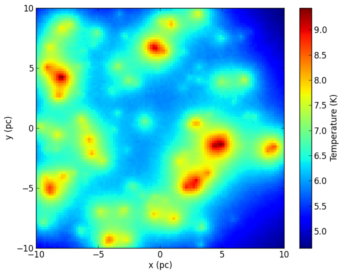
We can then use the get_quantities method described above to produce a
density-weighted temperature map collapsed in the z direction:
import numpy as np
import matplotlib.pyplot as plt

from hyperion.model import ModelOutput
from hyperion.util.constants import pc

# Read in the model
m = ModelOutput('quantity_cartesian.rtout')

# Extract the quantities
g = m.get_quantities()

# Get the wall positions in pc
xw, yw = g.x_wall / pc, g.y_wall / pc

# Make a 2-d grid of the wall positions (used by pcoloarmesh)
X, Y = np.meshgrid(xw, yw)

# Calculate the density-weighted temperature
weighted_temperature = (np.sum(g['temperature'][0].array
                               * g['density'][0].array, axis=2)
                        / np.sum(g['density'][0].array, axis=2))

# Make the plot
fig = plt.figure()
ax = fig.add_subplot(1, 1, 1)
c = ax.pcolormesh(X, Y, weighted_temperature)
ax.set_xlim(xw[0], xw[-1])
ax.set_xlim(yw[0], yw[-1])
ax.set_xlabel('x (pc)')
ax.set_ylabel('y (pc)')
cb = fig.colorbar(c)
cb.set_label('Temperature (K)')
fig.savefig('weighted_temperature_cartesian.png', bbox_inches='tight')
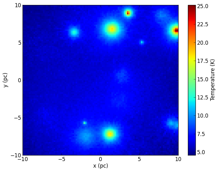
Of course, we can also plot individual slices:
fig = plt.figure()
ax = fig.add_subplot(1, 1, 1)
c = ax.pcolormesh(X, Y, g['temperature'][0].array[:, 49, :])
ax.set_xlim(xw[0], xw[-1])
ax.set_xlim(yw[0], yw[-1])
ax.set_xlabel('x (pc)')
ax.set_ylabel('y (pc)')
cb = fig.colorbar(c)
cb.set_label('Temperature (K)')
fig.savefig('sliced_temperature_cartesian.png', bbox_inches='tight')
Spherical polar grid example#
Polar grids are another interest case, because one might want to plot the result in polar or cartesian coordinates. To demonstrate this, we set up a simple example with a star surrounded by a flared disk:
from hyperion.model import AnalyticalYSOModel
from hyperion.util.constants import lsun, rsun, tsun, msun, au

# Initialize model and set up density grid
m = AnalyticalYSOModel()

# Set up the central source
m.star.radius = rsun
m.star.temperature = tsun
m.star.luminosity = lsun

# Set up a simple flared disk
d = m.add_flared_disk()
d.mass = 0.001 * msun
d.rmin = 0.1 * au
d.rmax = 100. * au
d.p = -1
d.beta = 1.25
d.h_0 = 0.01 * au
d.r_0 = au
d.dust = 'kmh_lite.hdf5'

# Specify that the specific energy and density are needed
m.conf.output.output_specific_energy = 'last'
m.conf.output.output_density = 'last'

# Set the number of photons
m.set_n_photons(initial=1000000, imaging=0)

# Set up the grid
m.set_spherical_polar_grid_auto(400, 300, 1)

# Use MRW and PDA
m.set_mrw(True)
m.set_pda(True)

# Write output and run model
m.write('quantity_spherical.rtin')
m.run('quantity_spherical.rtout', mpi=True)
Note
If you want to run this model you will need to download
the kmh_lite.hdf5 dust file into the
same directory as the script above (disclaimer: do not use this
dust file outside of these tutorials!).
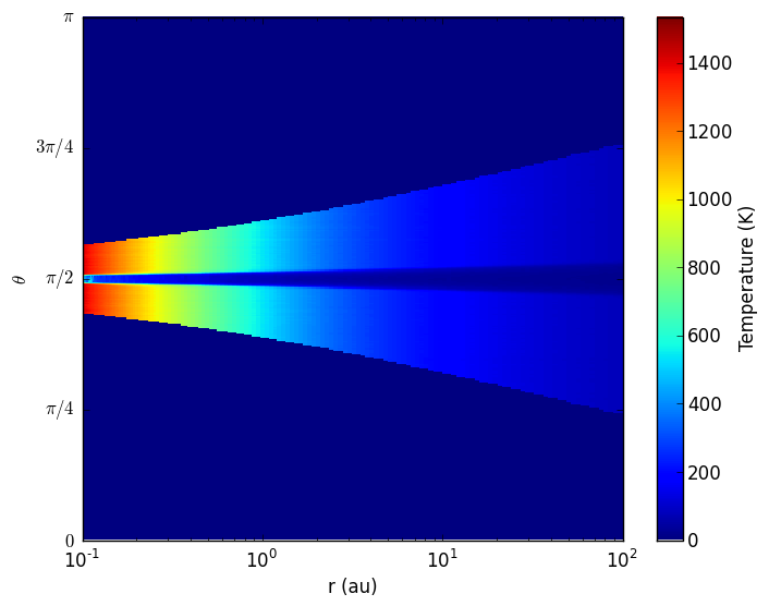
Making a plot of temperature in (r, theta) space is similar to before:
import numpy as np
import matplotlib.pyplot as plt

from hyperion.model import ModelOutput
from hyperion.util.constants import au

# Read in the model
m = ModelOutput('quantity_spherical.rtout')

# Extract the quantities
g = m.get_quantities()

# Get the wall positions for r and theta
rw, tw = g.r_wall / au, g.t_wall

# Make a 2-d grid of the wall positions (used by pcolormesh)
R, T = np.meshgrid(rw, tw)

# Make a plot in (r, theta) space
fig = plt.figure()
ax = fig.add_subplot(1, 1, 1)
c = ax.pcolormesh(R, T, g['temperature'][0].array[0, :, :])
ax.set_xscale('log')
ax.set_xlim(rw[1], rw[-1])
ax.set_ylim(tw[0], tw[-1])
ax.set_xlabel('r (au)')
ax.set_ylabel(r'$\theta$')
ax.set_yticks([np.pi, np.pi * 0.75, np.pi * 0.5, np.pi * 0.25, 0.])
ax.set_yticklabels([r'$\pi$', r'$3\pi/4$', r'$\pi/2$', r'$\pi/4$', r'$0$'])
cb = fig.colorbar(c)
cb.set_label('Temperature (K)')
fig.savefig('temperature_spherical_rt.png', bbox_inches='tight')
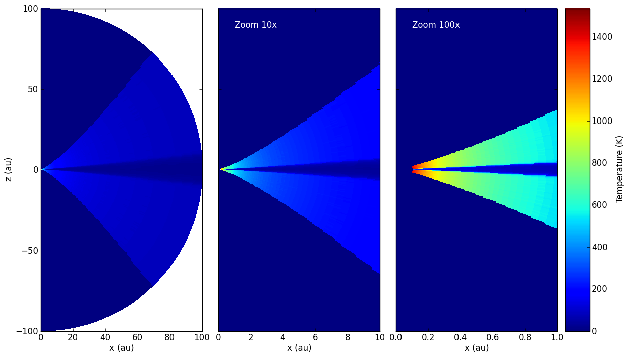
Making a plot in spherical coordinates instead is in fact also straightforward:
# Calculate the position of the cell walls in cartesian coordinates
R, T = np.meshgrid(rw, tw)
X, Z = R * np.sin(T), R * np.cos(T)

# Make a plot in (x, z) space for different zooms
fig = plt.figure(figsize=(16, 8))

ax = fig.add_axes([0.1, 0.1, 0.2, 0.8])
c = ax.pcolormesh(X, Z, g['temperature'][0].array[0, :, :])
ax.set_xlim(X.min(), X.max())
ax.set_ylim(Z.min(), Z.max())
ax.set_xlabel('x (au)')
ax.set_ylabel('z (au)')

ax = fig.add_axes([0.32, 0.1, 0.2, 0.8])
c = ax.pcolormesh(X, Z, g['temperature'][0].array[0, :, :])
ax.set_xlim(X.min() / 10., X.max() / 10.)
ax.set_ylim(Z.min() / 10., Z.max() / 10.)
ax.set_xlabel('x (au)')
ax.set_yticklabels('')
ax.text(0.1, 0.95, 'Zoom 10x', ha='left', va='center',
        transform=ax.transAxes, color='white')

ax = fig.add_axes([0.54, 0.1, 0.2, 0.8])
c = ax.pcolormesh(X, Z, g['temperature'][0].array[0, :, :])
ax.set_xlim(X.min() / 100., X.max() / 100)
ax.set_ylim(Z.min() / 100, Z.max() / 100)
ax.set_xlabel('x (au)')
ax.set_yticklabels('')
ax.text(0.1, 0.95, 'Zoom 100x', ha='left', va='center',
        transform=ax.transAxes, color='white')

ax = fig.add_axes([0.75, 0.1, 0.03, 0.8])
cb = fig.colorbar(c, cax=ax)
cb.set_label('Temperature (K)')

fig.savefig('temperature_spherical_xz.png', bbox_inches='tight')