Typical Analytical YSO Model

The following example model sets up the Class I model from Whitney et al (2003) For now, this model does not include the accretion luminosity, but this will be added in the future. First, we set up the model using the AnalyticalYSOModel class:

import numpy as np

from hyperion.model import AnalyticalYSOModel
from hyperion.util.constants import rsun, lsun, au, msun, yr, c

# Initalize the model
m = AnalyticalYSOModel()

# Read in stellar spectrum
wav, fnu = np.loadtxt('kt04000g+3.5z-2.0.ascii', unpack=True)
nu = c / (wav * 1.e-4)

# Set the stellar parameters
m.star.radius = 2.09 * rsun
m.star.spectrum = (nu, fnu)
m.star.luminosity = lsun
m.star.mass = 0.5 * msun

# Add a flared disk
disk = m.add_flared_disk()
disk.mass = 0.01 * msun
disk.rmin = 7 * m.star.radius
disk.rmax = 200 * au
disk.r_0 = m.star.radius
disk.h_0 = 0.01 * disk.r_0
disk.p = -1.0
disk.beta = 1.25
disk.dust = 'kmh_lite.hdf5'

# Add an Ulrich envelope
envelope = m.add_ulrich_envelope()
envelope.rc = disk.rmax
envelope.mdot = 5.e-6 * msun / yr
envelope.rmin = 7 * m.star.radius
envelope.rmax = 5000 * au
envelope.dust = 'kmh_lite.hdf5'

# Add a bipolar cavity
cavity = envelope.add_bipolar_cavity()
cavity.power = 1.5
cavity.theta_0 = 20
cavity.r_0 = envelope.rmax
cavity.rho_0 = 5e4 * 3.32e-24
cavity.rho_exp = 0.
cavity.dust = 'kmh_lite.hdf5'

# Use raytracing to improve s/n of thermal/source emission
m.set_raytracing(True)

# Use the modified random walk
m.set_mrw(True, gamma=2.)

# Set up grid
m.set_spherical_polar_grid_auto(399, 199, 1)

# Set up SED
sed = m.add_peeled_images(sed=True, image=False)
sed.set_viewing_angles(np.linspace(0., 90., 10), np.repeat(45., 10))
sed.set_wavelength_range(150, 0.02, 2000.)

# Set number of photons
m.set_n_photons(initial=1e6, imaging=1e6,
                raytracing_sources=1e4, raytracing_dust=1e6)

# Set number of temperature iterations and convergence criterion
m.set_n_initial_iterations(10)
m.set_convergence(True, percentile=99.0, absolute=2.0, relative=1.1)

# Write out file
m.write('class1_example.rtin')
m.run('class1_example.rtout', mpi=True)

Note

If you want to run this model you will need to download the kmh_lite.hdf5 dust file into the same directory as the script above (disclaimer: do not use this dust file outside of these tutorials!). You will also need the stellar photosphere model from here.

The model takes a few minutes to run on 12 processes (a little less than an hour in serial mode). We can then proceed for example to plotting the SED:

import matplotlib.pyplot as plt

from hyperion.model import ModelOutput
from hyperion.util.constants import pc

mo = ModelOutput('class1_example.rtout')
sed = mo.get_sed(aperture=-1, distance=140. * pc)

fig = plt.figure(figsize=(5, 4))
ax = fig.add_subplot(1, 1, 1)
ax.loglog(sed.wav, sed.val.transpose(), color='black')
ax.set_xlim(0.03, 2000.)
ax.set_ylim(2.e-15, 1e-8)
ax.set_xlabel(r'$\lambda$ [$\mu$m]')
ax.set_ylabel(r'$\lambda F_\lambda$ [ergs/cm$^2/s$]')
fig.savefig('class1_example_sed.png', bbox_inches='tight')

which gives:

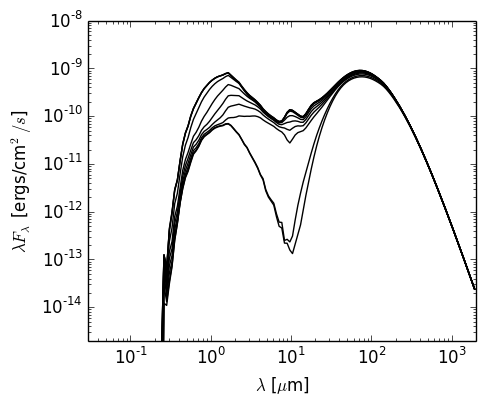
which is almost identical to the bottom left panel of Figure 3a of Whitney et al (2003) (the differences being due to slightly different dust properties).