How to set the luminosity for an external radiation field

Two source types, ExternalSphericalSource and ExternalBoxSource are available, and can be used to simulate an external radiation field (such as the interstellar radiation field or I). One of the tricky parameters to set is the luminosity, because one often knows what the mean intensity of the interstellar radiation field should be, but not the total luminosity emitted from a spherical or box surface.

From empirical tests, we find that if one wants a particular value of (the mean intensity integrated over frequency), then the luminosity should be set to where is the area of the external source. We can check this using, as an example, the ISRF model from Mathis, Mezger, and Panagia (hereafter MMP; 1983), who find

in the solar neighborhood.

We now set up a model with a spherical grid extending to 1pc in radius, with the spectrum given by MMP83:

import numpy as np

from hyperion.model import Model
from hyperion.util.constants import pc, c

# The following value is taken from Mathis, Mezger, and Panagia (1983)
FOUR_PI_JNU = 0.0217

# Initialize model
m = Model()

# Set up grid
m.set_spherical_polar_grid([0., 1.001 * pc],
                           [0., np.pi],
                           [0., 2. * np.pi])

# Read in MMP83 spectrum
wav, jlambda = np.loadtxt('mmp83.txt', unpack=True)
nu = c / (wav * 1.e-4)
jnu = jlambda * wav / nu

# Set up the source - note that the normalization of the spectrum is not
# important - the luminosity is set separately.
s = m.add_external_spherical_source()
s.radius = pc
s.spectrum = (nu, jnu)
s.luminosity = np.pi * pc * pc * FOUR_PI_JNU

# Add an inside observer with an all-sky camera
image = m.add_peeled_images(sed=False, image=True)
image.set_inside_observer((0., 0., 0.))
image.set_image_limits(180., -180., -90., 90.)
image.set_image_size(256, 128)
image.set_wavelength_range(100, 0.01, 1000.)

# Use raytracing for high signal-to-noise
m.set_raytracing(True)

# Don't compute the temperature
m.set_n_initial_iterations(0)

# Only include photons from the source (since there is no dust)
m.set_n_photons(imaging=0,
                raytracing_sources=10000000,
                raytracing_dust=0)

# Write out and run the model
m.write('example_isrf.rtin')
m.run('example_isrf.rtout')

To run this model, you will need the mmp83.txt file which contains the spectrum of the interstellar radiation field. We have set up an observer inside the grid to make an all-sky integrated intensity map:

import numpy as np
import matplotlib.pyplot as plt

from hyperion.model import ModelOutput
from hyperion.util.integrate import integrate_loglog

# Use LaTeX for plots
plt.rc('text', usetex=True)

# Open the output file
m = ModelOutput('example_isrf.rtout')

# Get an all-sky flux map
image = m.get_image(units='ergs/cm^2/s/Hz', inclination=0)

# Compute the frequency-integrated flux
fint = np.zeros(image.val.shape[:-1])
for (j, i) in np.ndindex(fint.shape):
    fint[j, i] = integrate_loglog(image.nu, image.val[j, i, :])

# Find the area of each pixel
l = np.radians(np.linspace(180., -180., fint.shape[1] + 1))
b = np.radians(np.linspace(-90., 90., fint.shape[0] + 1))
dl = l[1:] - l[:-1]
db = np.sin(b[1:]) - np.sin(b[:-1])
DL, DB = np.meshgrid(dl, db)
area = np.abs(DL * DB)

# Compute the intensity
intensity = fint / area

# Intitialize plot
fig = plt.figure()
ax = fig.add_subplot(1, 1, 1, projection='aitoff')

# Show intensity
image = ax.pcolormesh(l, b, intensity, cmap=plt.cm.gist_heat, vmin=0.0, vmax=0.0025)

# Add mean intensity
four_pi_jnu = round(np.sum(intensity * area), 4)
fig.text(0.40, 0.15, r"$4\pi J = %6.4f$ "
                     r"${\rm erg\,cm^{-2}\,s^{-1}}$" % four_pi_jnu, size=14)

# Add a colorbar
cax = fig.add_axes([0.92, 0.25, 0.02, 0.5])
fig.colorbar(image, cax=cax)

# Add title and improve esthetics
ax.set_title(r"Integrated intensity in a given pixel "
             r"(${\rm erg\,cm^{-2}\,s^{-1}\,ster^{-1}}$)", size=12, y=1.1)
ax.grid()
ax.tick_params(axis='both', which='major', labelsize=10)
cax.tick_params(axis='both', which='major', labelsize=10)

# Save the plot
fig.savefig('isrf_intensity.png', bbox_inches='tight')

which gives:

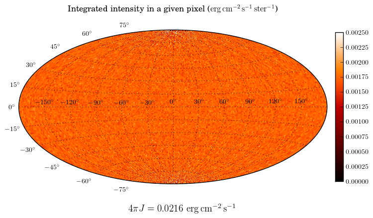
As we can see, the value for is almost identical to the value we initially used above.