How to efficiently compute pure scattering models#
In some cases, for example if the wavelength is short enough, it is possible to ignore dust emission when computing images. In such cases, we can make Hyperion run faster by disabling the temperature calculation as described in Scattered-light images, and also by producing images only at select wavelengths using Monochromatic radiative transfer. The following model demonstrates how to make an image of the central region of a flared disk in order to image the inner rim:
from hyperion.model import AnalyticalYSOModel
from hyperion.util.constants import au, lsun, rsun, tsun, msun

# Initialize model
m = AnalyticalYSOModel()

# Set up star
m.star.radius = 1.5 * rsun
m.star.temperature = tsun
m.star.luminosity = lsun

# Set up disk
d = m.add_flared_disk()
d.rmin = 10 * rsun
d.rmax = 30. * au
d.mass = 0.01 * msun
d.p = -1
d.beta = 1.25
d.r_0 = 10. * au
d.h_0 = 0.4 * au
d.dust = 'kmh_lite.hdf5'

# Set up grid
m.set_spherical_polar_grid_auto(400, 100, 1)

# Don't compute temperatures
m.set_n_initial_iterations(0)

# Don't re-emit photons
m.set_kill_on_absorb(True)

# Use raytracing (only important for source here, since no dust emission)
m.set_raytracing(True)

# Compute images using monochromatic radiative transfer
m.set_monochromatic(True, wavelengths=[1.])

# Set up image
i = m.add_peeled_images()
i.set_image_limits(-13 * rsun, 13 * rsun, -13. * rsun, 13 * rsun)
i.set_image_size(256, 256)
i.set_viewing_angles([60.], [20.])
i.set_wavelength_index_range(1, 1)
i.set_stokes(True)

# Set number of photons
m.set_n_photons(imaging_sources=10000000, imaging_dust=0,
                raytracing_sources=100000, raytracing_dust=0)

# Write out the model and run it in parallel
m.write('pure_scattering.rtin')
m.run('pure_scattering.rtout', mpi=True)
Note
If you want to run this model you will need to download
the kmh_lite.hdf5 dust file into the
same directory as the script above (disclaimer: do not use this
dust file outside of these tutorials!).
Once this model has run, we can make a plot of the image (including a linear polarization map):
import matplotlib.pyplot as plt
from hyperion.model import ModelOutput
from hyperion.util.constants import pc

mo = ModelOutput('pure_scattering.rtout')

image_fnu = mo.get_image(inclination=0, units='MJy/sr', distance=300. * pc)
image_pol = mo.get_image(inclination=0, stokes='linpol')

fig = plt.figure(figsize=(8, 8))

# Make total intensity sub-plot

ax = fig.add_axes([0.1, 0.3, 0.4, 0.4])
ax.imshow(image_fnu.val[:, :, 0], extent=[-13, 13, -13, 13],
          interpolation='none', cmap=plt.cm.gist_heat,
          origin='lower', vmin=0., vmax=4e9)
ax.set_xlim(-13., 13.)
ax.set_ylim(-13., 13.)
ax.set_xlabel("x (solar radii)")
ax.set_ylabel("y (solar radii)")
ax.set_title("Surface brightness")

# Make linear polarization sub-plot

ax = fig.add_axes([0.51, 0.3, 0.4, 0.4])
im = ax.imshow(image_pol.val[:, :, 0] * 100., extent=[-13, 13, -13, 13],
               interpolation='none', cmap=plt.cm.gist_heat,
               origin='lower', vmin=0., vmax=100.)
ax.set_xlim(-13., 13.)
ax.set_ylim(-13., 13.)
ax.set_xlabel("x (solar radii)")
ax.set_title("Linear Polarization")
ax.set_yticklabels('')

axcb = fig.add_axes([0.92, 0.3, 0.02, 0.4])
cb=plt.colorbar(im, cax=axcb)
cb.set_label('%')
fig.savefig('pure_scattering_inner_disk.png', bbox_inches='tight')
which gives:
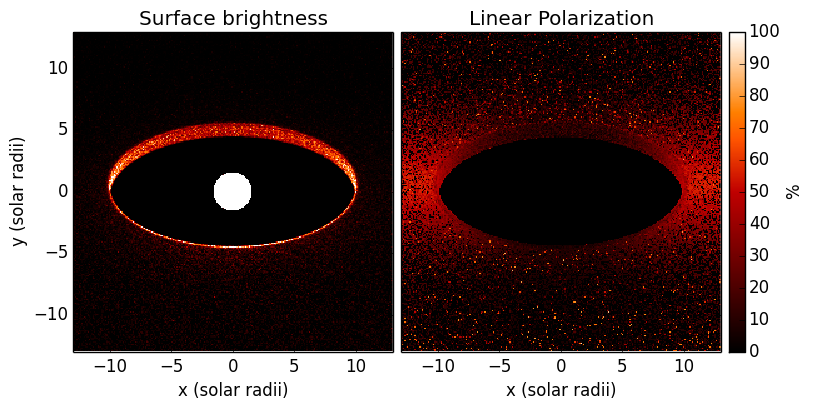
This model takes under 4 minutes to run on 8 cores, which is less than would normally be required to produce an image with this signal-to-noise in scattered light.