Plotting and writing images

As mentioned in Plotting and writing out SEDs, the output files from the radiative transfer code are in the HDF5 file format, and can therefore be accessed directly from most programming/scripting languages. However, in most cases it is easiest to use the Hyperion Python library to extract the required information and write it out to files. In this tutorial, we learn how to write out images to FITS files (for an example of writing out SEDs, see Plotting and writing out SEDs).

Example model

In this example, we set up a simple model that consists of a cube of constant density, with a point source shining isotropically. A denser cube then causes some of the emission to be blocked, and casts a shadow:

import numpy as np

from hyperion.model import Model
from hyperion.util.constants import pc, lsun

# Initialize model
m = Model()

# Set up 64x64x64 cartesian grid
w = np.linspace(-pc, pc, 64)
m.set_cartesian_grid(w, w, w)

# Add density grid with constant density and add a higher density cube inside to
# cause a shadow.
density = np.ones(m.grid.shape) * 1e-21
density[26:38, 26:38, 26:38] = 1.e-18
m.add_density_grid(density, 'kmh_lite.hdf5')

# Add a point source in the center
s = m.add_point_source()
s.position = (0.4 * pc, 0., 0.)
s.luminosity = 1000 * lsun
s.temperature = 6000.

# Add multi-wavelength image for a single viewing angle
image = m.add_peeled_images(sed=False, image=True)
image.set_wavelength_range(20, 1., 1000.)
image.set_viewing_angles([60.], [80.])
image.set_image_size(400, 400)
image.set_image_limits(-1.5 * pc, 1.5 * pc, -1.5 * pc, 1.5 * pc)

# Set runtime parameters
m.set_n_initial_iterations(5)
m.set_raytracing(True)
m.set_n_photons(initial=4e6, imaging=4e7,
                raytracing_sources=1, raytracing_dust=1e7)

# Write out input file
m.write('simple_cube.rtin')
m.run('simple_cube.rtout', mpi=True)

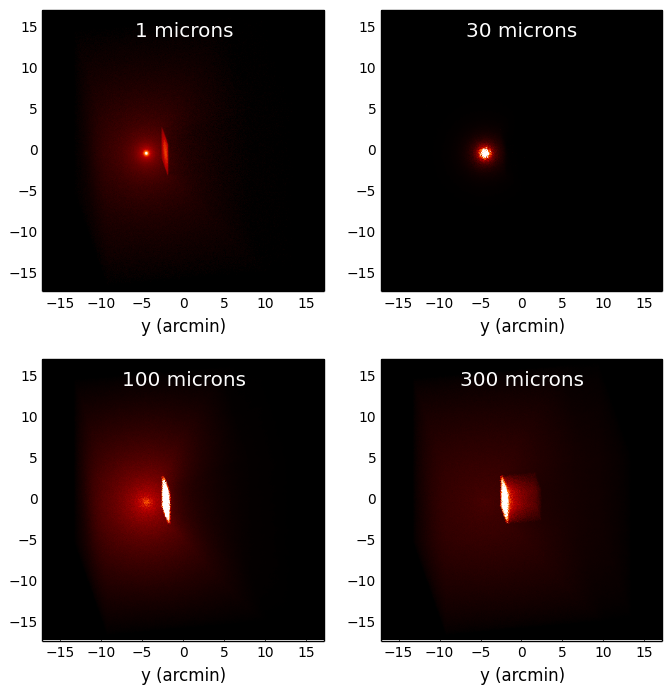
Plotting images

Note

If you have never used Matplotlib before, you can first take a look at the An introduction to Matplotlib tutorial.

The first step is to extract the image cube from the output file (simple_cube.rtout). This step is described in detail in Post-processing models. We can make a plot of the surface brightness

import numpy as np
import matplotlib.pyplot as plt

from hyperion.model import ModelOutput
from hyperion.util.constants import pc

# Open the model
m = ModelOutput('simple_cube.rtout')

# Extract the image for the first inclination, and scale to 300pc. We
# have to specify group=1 as there is no image in group 0.
image = m.get_image(inclination=0, distance=300 * pc, units='MJy/sr')

# Open figure and create axes
fig = plt.figure(figsize=(8, 8))

# Pre-set maximum for colorscales
VMAX = {}
VMAX[1] = 10.
VMAX[30] = 100.
VMAX[100] = 2000.
VMAX[300] = 2000.

# We will now show four sub-plots, each one for a different wavelength
for i, wav in enumerate([1, 30, 100, 300]):

    ax = fig.add_subplot(2, 2, i + 1)

    # Find the closest wavelength
    iwav = np.argmin(np.abs(wav - image.wav))

    # Calculate the image width in arcseconds given the distance used above
    w = np.degrees((1.5 * pc) / image.distance) * 60.

    # This is the command to show the image. The parameters vmin and vmax are
    # the min and max levels for the colorscale (remove for default values).
    ax.imshow(np.sqrt(image.val[:, :, iwav]), vmin=0, vmax=np.sqrt(VMAX[wav]),
              cmap=plt.cm.gist_heat, origin='lower', extent=[-w, w, -w, w])

    # Finalize the plot
    ax.tick_params(axis='both', which='major', labelsize=10)
    ax.set_xlabel('x (arcmin)')
    ax.set_xlabel('y (arcmin)')
    ax.set_title(str(wav) + ' microns', y=0.88, x=0.5, color='white')

fig.savefig('simple_cube_plot.png', bbox_inches='tight')

This script produces the following plot:

Writing out images

Writing out images to text files does not make much sense, so in this section we see how to write out images extracted from the radiative transfer code results to a FITS file, and add WCS information. Once a 2D image or 3D wavelength cube have been extracted as shown in Plotting images, we can write them out to a FITS file using Astropy:

from astropy.io import fits

from hyperion.model import ModelOutput
from hyperion.util.constants import pc

# Retrieve image cube as before
m = ModelOutput('simple_cube.rtout')
image = m.get_image(inclination=0, distance=300 * pc, units='MJy/sr')

# The image extracted above is a 3D array. We can write it out to FITS.
# We need to swap some of the directions around so as to be able to use
# the ds9 slider to change the wavelength of the image.
fits.writeto('simple_cube.fits', image.val.swapaxes(0, 2).swapaxes(1, 2),
             clobber=True)

# We can also just output one of the wavelengths
fits.writeto('simple_cube_slice.fits', image.val[:, :, 1], clobber=True)

Writing out images with WCS information

Adding World Coordinate System (WCS) information is easy using Astropy:

import numpy as np

from astropy.io import fits
from astropy.wcs import WCS

from hyperion.model import ModelOutput
from hyperion.util.constants import pc

# Retrieve image cube as before
m = ModelOutput('simple_cube.rtout')
image = m.get_image(inclination=0, distance=300 * pc, units='MJy/sr')

# Initialize WCS information
wcs = WCS(naxis=2)

# Use the center of the image as projection center
wcs.wcs.crpix = [image.val.shape[1] / 2. + 0.5,
                 image.val.shape[0] / 2. + 0.5]

# Set the coordinates of the image center
wcs.wcs.crval = [233.4452, 1.2233]

# Set the pixel scale (in deg/pix)
scale = np.degrees(3. * pc / image.val.shape[0] / image.distance)
wcs.wcs.cdelt = [-scale, scale]

# Set the coordinate system
wcs.wcs.ctype = ['GLON-CAR', 'GLAT-CAR']

# And produce a FITS header
header = wcs.to_header()

# We can also just output one of the wavelengths
fits.writeto('simple_cube_slice_wcs.fits', image.val[:, :, 1],
             header=header, clobber=True)

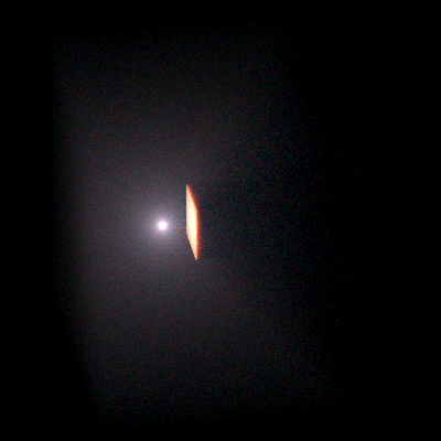
Making 3-color images

Making 3-color images is possible using the Python Imaging Library. The following example demonstrates how to produce a 3-color PNG of the above model using the scattered light wavelengths:

import numpy as np
from PIL import Image

from hyperion.model import ModelOutput
from hyperion.util.constants import pc

m = ModelOutput('simple_cube.rtout')
image = m.get_image(inclination=0, distance=300 * pc, units='MJy/sr')

# Extract the slices we want to use for red, green, and blue
r = image.val[:, :, 17]
g = image.val[:, :, 18]
b = image.val[:, :, 19]

# Now we need to rescale the values we want to the range 0 to 255, clip values
# outside the range, and convert to unsigned 8-bit integers. We also use a sqrt
# stretch (hence the ** 0.5)

r = np.clip((r / 0.5) ** 0.5 * 255., 0., 255.)
r = np.array(r, dtype=np.uint8)

g = np.clip((g / 2) ** 0.5 * 255., 0., 255.)
g = np.array(g, dtype=np.uint8)

b = np.clip((b / 4.) ** 0.5 * 255., 0., 255.)
b = np.array(b, dtype=np.uint8)

# We now convert to image objects
image_r = Image.fromarray(r)
image_g = Image.fromarray(g)
image_b = Image.fromarray(b)

# And finally merge into a single 3-color image
img = Image.merge("RGB", (image_r, image_g, image_b))

# By default, the image will be flipped, so we need to fix this
img = img.transpose(Image.FLIP_TOP_BOTTOM)

img.save('simple_cube_rgb.png')

which gives:

Alternatively, you can write out the required images to FITS format, then use the make_rgb_image function in APLpy to make the 3-color images.