Plotting and writing out SEDs

So you’ve run a model with SEDs, and you now want to plot them or write the out to files. The plotting library used in this tutorial is Matplotlib but there is no reason why you can’t use another. The examples below get you to write Python scripts, but you can also run these interactively in python or ipython if you like.

Example model

As an example, let’s set up a simple model of a star with a blackbody spectrum surrounded by a flared disk using the AnalyticalYSOModel class.

import numpy as np

from hyperion.model import AnalyticalYSOModel
from hyperion.util.constants import rsun, au, msun, sigma

# Initalize the model
m = AnalyticalYSOModel()

# Set the stellar parameters
m.star.radius = 2. * rsun
m.star.temperature = 4000.
m.star.luminosity = 4 * (2. * rsun) ** 2 * sigma * 4000 ** 4

# Add a flared disk
disk = m.add_flared_disk()
disk.mass = 0.01 * msun
disk.rmin = 10 * m.star.radius
disk.rmax = 200 * au
disk.r_0 = m.star.radius
disk.h_0 = 0.01 * disk.r_0
disk.p = -1.0
disk.beta = 1.25
disk.dust = 'kmh_lite.hdf5'

# Use raytracing to improve s/n of thermal/source emission
m.set_raytracing(True)

# Use the modified random walk
m.set_mrw(True, gamma=2.)

# Set up grid
m.set_spherical_polar_grid_auto(399, 199, 1)

# Set up SED for 10 viewing angles
sed = m.add_peeled_images(sed=True, image=False)
sed.set_viewing_angles(np.linspace(0., 90., 10), np.repeat(45., 10))
sed.set_wavelength_range(150, 0.02, 2000.)
sed.set_track_origin('basic')

# Set number of photons
m.set_n_photons(initial=1e5, imaging=1e6,
                raytracing_sources=1e4, raytracing_dust=1e6)

# Set number of temperature iterations
m.set_n_initial_iterations(5)

# Write out file
m.write('class2_sed.rtin')
m.run('class2_sed.rtout', mpi=True)

Note that the subsequent plotting code applies to any model, not just AnalyticalYSOModel models.

Plotting SEDs

Note

If you have never used Matplotlib before, you can first take a look at the An introduction to Matplotlib tutorial.

Total flux

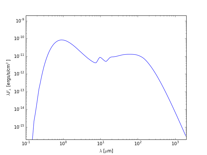
Once the above model has run, we are ready to make a simple SED plot. The first step is to extract the SED from the output file from the radiation transfer code. This step is described in detail in Post-processing models. Combining this with what we learned above about making plots, we can write scripts that will fetch SEDs and plot them. For example, if we want to plot an SED for the first inclination and the largest aperture, we can do:

import matplotlib.pyplot as plt

from hyperion.model import ModelOutput
from hyperion.util.constants import pc

# Open the model
m = ModelOutput('class2_sed.rtout')

# Create the plot
fig = plt.figure()
ax = fig.add_subplot(1, 1, 1)

# Extract the SED for the smallest inclination and largest aperture, and
# scale to 300pc. In Python, negative indices can be used for lists and
# arrays, and indicate the position from the end. So to get the SED in the
# largest aperture, we set aperture=-1.
sed = m.get_sed(inclination=0, aperture=-1, distance=300 * pc)

# Plot the SED. The loglog command is similar to plot, but automatically
# sets the x and y axes to be on a log scale.
ax.loglog(sed.wav, sed.val)

# Add some axis labels (we are using LaTeX here)
ax.set_xlabel(r'$\lambda$ [$\mu$m]')
ax.set_ylabel(r'$\lambda F_\lambda$ [ergs/s/cm$^2$]')

# Set view limits
ax.set_xlim(0.1, 2000.)
ax.set_ylim(2.e-16, 2.e-9)

# Write out the plot
fig.savefig('class2_sed_plot_single.png')

This script produces the following plot:

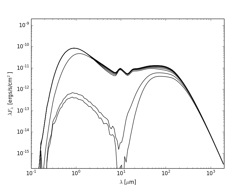
Now let’s say that we want to plot the SED for all inclinations. We can either call get_sed() and loglog once for each inclination, or call it once with inclination='all' and then call only loglog once for each inclination:

import matplotlib.pyplot as plt

from hyperion.model import ModelOutput
from hyperion.util.constants import pc

m = ModelOutput('class2_sed.rtout')

fig = plt.figure()
ax = fig.add_subplot(1, 1, 1)

# Extract all SEDs
sed = m.get_sed(inclination='all', aperture=-1, distance=300 * pc)

# Plot SED for each inclination
for i in range(sed.val.shape[0]):
    ax.loglog(sed.wav, sed.val[i, :], color='black')

ax.set_xlabel(r'$\lambda$ [$\mu$m]')
ax.set_ylabel(r'$\lambda F_\lambda$ [ergs/s/cm$^2$]')
ax.set_xlim(0.1, 2000.)
ax.set_ylim(2.e-16, 2.e-9)
fig.savefig('class2_sed_plot_incl.png')

This script produces the following plot:

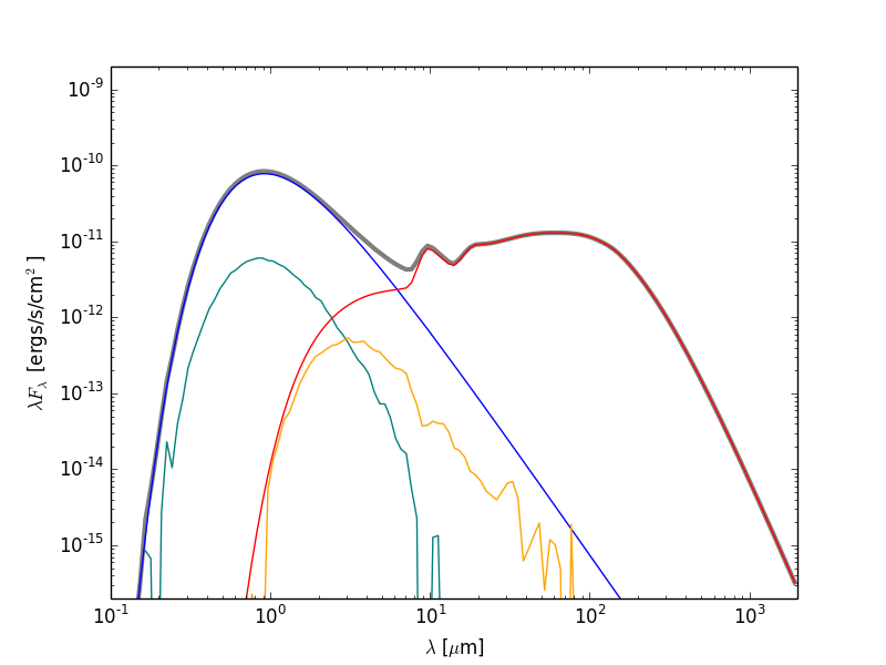
Individual SED components

Now let’s do something a little more fancy. Assuming that you set up the SEDs with photon tracking:

sed.set_track_origin('basic')

or:

sed.set_track_origin('detailed')

you can plot the individual components. Notice that we included the former in the model at the top of this page, so we can make use of it here to plot separate components of the SED.

The following example retrieves each separate components, and plots it in a different color:

import matplotlib.pyplot as plt

from hyperion.model import ModelOutput
from hyperion.util.constants import pc

m = ModelOutput('class2_sed.rtout')

fig = plt.figure()
ax = fig.add_subplot(1, 1, 1)

# Total SED
sed = m.get_sed(inclination=0, aperture=-1, distance=300 * pc)
ax.loglog(sed.wav, sed.val, color='black', lw=3, alpha=0.5)

# Direct stellar photons
sed = m.get_sed(inclination=0, aperture=-1, distance=300 * pc,
                       component='source_emit')
ax.loglog(sed.wav, sed.val, color='blue')

# Scattered stellar photons
sed = m.get_sed(inclination=0, aperture=-1, distance=300 * pc,
                       component='source_scat')
ax.loglog(sed.wav, sed.val, color='teal')

# Direct dust photons
sed = m.get_sed(inclination=0, aperture=-1, distance=300 * pc,
                       component='dust_emit')
ax.loglog(sed.wav, sed.val, color='red')

# Scattered dust photons
sed = m.get_sed(inclination=0, aperture=-1, distance=300 * pc,
                       component='dust_scat')
ax.loglog(sed.wav, sed.val, color='orange')


ax.set_xlabel(r'$\lambda$ [$\mu$m]')
ax.set_ylabel(r'$\lambda F_\lambda$ [ergs/s/cm$^2$]')
ax.set_xlim(0.1, 2000.)
ax.set_ylim(2.e-16, 2.e-9)
fig.savefig('class2_sed_plot_components.png')

This script produces the following plot:

Writing out SEDs

Note

If you have never written text files from Python before, you can first take a look at the Writing files in Python tutorial.

The output files from the radiative transfer code are in the HDF5 file format, and can therefore be accessed directly from most programming/scripting languages. However, in many cases it might be most convenient to write a small Python script to extract the required information and to write it out to files that can then be read in to other tools.

For instance, you may want to write out the SEDs to ASCII files. To do this, the first step, as for plotting (see Plotting SEDs above) is to extract the SED from the output file from the radiation transfer code. This step is also described in detail in Post-processing models. Once we have extracted an SED we can write a script that will write it out to disk. For example, if we want to write out the SED for the first inclination and the largest aperture from the Example Model, we can do:

import numpy as np

from hyperion.model import ModelOutput
from hyperion.util.constants import pc

m = ModelOutput('class2_sed.rtout')
sed = m.get_sed(inclination=0, aperture=-1, distance=300 * pc)
np.savetxt('sed.txt', list(zip(sed.wav, sed.val)), fmt="%11.4e %11.4e")

This script produces a file that looks like:

 1.9247e+03  3.2492e-16
 1.7825e+03  4.6943e-16
 1.6508e+03  6.7731e-16
 1.5288e+03  9.7580e-16
 1.4159e+03  1.4036e-15
 1.3113e+03  2.0154e-15
 1.2144e+03  2.8884e-15
 1.1247e+03  4.1310e-15
...