Preparing dust properties

Arguably one of the most important inputs to the model are the dust properties. At this time, Hyperion supports anisotropic wavelength-dependent scattering of randomly oriented grains, using a 4-element Mueller matrix (Chandrasekhar 1960; Code & Whitney 1995). See Section 2.1.3 of Robitaille (2011) for more details.

Note

Because the choice of a dust model is very important for the model, no ‘default’ dust models are provided with Hyperion, as there is no single sensible default. Instead, you can set up any dust model using the instructions below. In future, a database of published and common dust models will be provided. If you are not sure which dust model to use, or are not familiar with opacities, albedos, and scattering phase functions, you are strongly encouraged to team up with someone who is an expert on the topic of dust, as this should not be left to chance!

There are several ways to set up the dust properties that you want to use, and these are detailed in sections below. In all cases, setting up the dust models is done by first creating an instance of a specific dust class, then setting the properties, and optionally writing out the dust properties to a file:

from hyperion.dust import SphericalDust
d = SphericalDust()
< set dust properties here >
d.write('mydust.hdf5')

Note

Carefully look at the warnings that are raised when writing the dust file, as these may indicate issues that will have an impact on the radiative transfer. See Common warnings for more details.

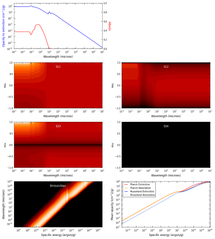
It is also possible to plot the dust properties:

d.plot('mydust.png')

which gives a plot that can be used to get an overview of all the dust properties:

Important note on units

In all of the following sections, quantities should be specified in the cgs system of units (e.g. for the opacities). Whether the opacities are specified per unit mass of dust or gas is not important, as long as the densities specified when setting up the geometry are consistent. For example, if the opacities are specified per unit dust mass, the densities specified when setting up the model should be dust densities.

Dust with isotropic scattering

Creating a dust object with isotropic scattering properties is very simple. First, import the IsotropicDust class:

from hyperion.dust import IsotropicDust

and create and instance of the class by specifying the frequency, albedo, and opacity to extinction (absorption + scattering):

d = IsotropicDust(nu, albedo, chi)

where nu, albedo, and chi should be specified as lists or 1-d Numpy arrays, and nu should be monotonically increasing. The albedo values should all be in the range 0 to 1, and the chi values should be positive. The scattering matrix elements will be set to give isotropic scattering, and the emissivities and mean opacities will be set assuming local thermodynamic equilibrium.

Dust with Henyey-Greenstein scattering

Creating a dust object with Henyey-Greenstein scattering properties is very similar to isotropic scattering, with the exception that the scattering parameters have to be specified. The scattering is anisotropic, and the phase function is defined by analytical functions (Henyey & Greenstein, 1941).

First, import the HenyeyGreensteinDust class:

from hyperion.dust import HenyeyGreensteinDust

and create an instance of the class by specifying the frequency, albedo, opacity to extinction (absorption + scattering), and the anisotropy factor and the maximum polarization:

d = HenyeyGreensteinDust(nu, albedo, chi, g, p_lin_max)

where nu, albedo, chi, g and p_lin_max should be specified as lists or 1-d Numpy arrays, and nu should be monotonically increasing. The albedo values should all be in the range 0 to 1, and the chi values should be positive. The scattering matrix elements will be set to give the correct phase function for the scattering properties specified, and the emissivities and mean opacities will be set assuming local thermodynamic equilibrium.

Fully customized 4-element dust

While the Henyey-Greenstein scattering phase function allows for anisotropic scattering, it approximates the phase function by analytical equations. In some cases, it is desirable to instead use the full numerical phase function which can be arbitrarily complex.

To set up a fully customized 4-element dust model, first import the SphericalDust class (this actually refers to any kind of dust that would produce a 4-element scattering matrix, including randomly oriented non-spherical grains):

from hyperion.dust import SphericalDust

Then create an instance of this class:

d = SphericalDust()

Now that you have a dust ‘object’, you will need to set the optical properties of the dust, which include the albedo and extinction coefficient (in cgs) as a function of frequency (in Hz):

d.optical_properties.nu = nu
d.optical_properties.albedo = albedo
d.optical_properties.chi = chi

where nu, albedo, and chi should be specified as lists or 1-d Numpy arrays, and nu should be monotonically increasing. The albedo values should all be in the range 0 to 1, and the chi values should be positive.

Once these basic properties are set, you will need to set the scattering properties by setting the matrix elements. These should be specified as a function of the cosine of the scattering angle, mu. The values of mu should be specified as a 1-d Numpy array:

d.optical_properties.mu = mu

Once nu and mu are set, the values of the scattering matrix elements can be set. These are stored in variables named using the convention of Code & Whitney (1995): P1 (equivalent to S11), P2 (equivalent to S12), P3 (equivalent to S44), and P4 (equivalent to -S34). Each of these variables should be specified as a 2-d array with dimensions (n_nu, n_mu), where n_nu is the number of frequencies, and n_mu is the number of values of the cosine of the scattering angle:

d.optical_properties.P1 = P1
d.optical_properties.P2 = P2
d.optical_properties.P3 = P3
d.optical_properties.P4 = P4

Alternatively, it is possible to call:

d.optical_properties.initialize_scattering_matrix()

After which P1, P2, P3, and P4 will be set to arrays with the right dimensions, and with all values set to zero. You could for example set up an isotropic scattering matrix by setting the values of the arrays:

d.optical_properties.P1[:, :] = 1.
d.optical_properties.P2[:, :] = 0.
d.optical_properties.P3[:, :] = 1.
d.optical_properties.P4[:, :] = 0.

If nothing else is specified, the dust emissivity will be set assuming local thermodynamic equilibrium (i.e. it will be set to the opacity to absorption times Planck functions).

Emissivities

By default, emissivities and mean opacities will be calculated under the assumption of local thermodynamic equilibrium for 1200 dust temperatures between 0.1 and 100000K, but this can be customized, as described below.

LTE emissivities

To set the LTE emissivities manually, you can call the set_lte_emissivities method. For example, to calculate the emissivities for 1000 temperatures between 0.1 and 2000K, you can do:

d.set_lte_emissivities(n_temp=1000,
                       temp_min=0.1,
                       temp_max=2000.)

The more temperatures the emissivities are calculated for, the more accurate the radiative transfer (Hyperion interpolates between emissivities, rather the picking the closest one) but the slower the dust file will be to generate and read into Hyperion.

Custom emissivities

If you want to specify fully customized emissivities as a function of specific energy, you can instead do this by directly accessing the variables, which are stored as attributes to d.emissivities, i.e.:

d.emissivities.nu
d.emissivities.var
d.emissivities.jnu
d.emissivities.var_name

The attribute nu should be set to a 1-d array giving the frequencies that the emissivities are specified for, var should be set to another 1-d array containing the values of the specific energy the emissivities are defined for, and jnu should be set to a 2-d array with dimensions (len(nu), len(var)) giving the emissivities. In addition, you will need to set var_name to 'specific_energy' (in future, other kinds of emissivity variables may be supported). For example, to set a constant emissivity as a function of frequency and specific energy, you can do:

d.emissivities.nu = np.logspace(8., 16., 100)  # 100 values between 10^8 and 10^16
d.emissivities.var = np.logspace(-2., 8., 20)  # 20 values of the specific energy
                                               # between 10^-2 and 10^8
d.emissivities.jnu = np.ones(100, 20)  # constant emissivities
d.emissivities.var_name = 'specific_energy'

Extrapolating optical properties

In some cases (see e.g. Common warnings) it can be necessary to extrapolate the dust properties to shorter and/or longer wavelengths. While it would be preferable to do this extrapolation properly before passing the values to the dust objects, in some cases the extrapolation is relatively straightforward, and you can make use of the following extrapolation convenience functions:

d.optical_properties.extrapolate_wav(0.1, 1000)
d.optical_properties.extrapolate_nu(1.e5, 1.e15)

In the first case, the extrapolation is done by specifying wavelengths in microns, and in the second case by specifying the frequency (in Hz).

The extrapolation is done in the following way:

• The opacity to extinction (chi) is extrapolated by fitting a power-law to the opacities at the two highest frequencies and following that power law, and similarly at the lowest frequencies. This ensures that the slope of the opacity remains constant.
• The albedo is extrapolated by assuming that the albedo is constant outside the original range, and is set to the same value as the values for the lowest and highest frequencies.
• The scattering matrix is extrapolated similarly to the albedo, by simply extending the values for the lowest and highest frequencies to the new frequency range.

The plots shown higher up on this page have made use of these extrapolation methods.

Common warnings

One of the most common warnings when computing the LTE emissivities or writing out a dust file is the following:

WARNING: Planck function for lowest temperature not completely covered by opacity function
WARNING: Planck function for highest temperature not completely covered by opacity function

The LTE emissivity is set to , so you need to ensure that the opacity is defined over a frequency large enough to allow this to be calculated from the lowest to the highest temperatures used for the LTE emissivities. The default range is quite large (0.1 to 100000K) so you can either reduce this range (see LTE emissivities) or you should define the optical properties over a larger frequency range (see Extrapolating optical properties for one way to do this).

More specifically, the frequency range should extend almost three orders of magnitude above the peak frequency for the coldest temperature, and one order of magnitude below the peak frequency for the hottest temperature. For the default temperature range for the LTE emissivities (0.1 to 100000K), this means going from about 5e7 to 5e16Hz (or 0.5nm to 5m) which is a huge frequency range, over which dust properties are often not known. However, in most cases, a sensible extrapolation of the properties you have should be fine - the plots shown higher up on this page show the values extrapolated to the required range. If you restrict yourself to a smaller temperature range (e.g. 3 to 1600K) you can also reduce the required range significantly.

Note

If you do not fix this warning, the normalization of the emissivities will be off, and the results from the radiative transfer may be incorrect!

Writing dust files without the Python library

If for any reason you wish to write the HDF5 dust files directly without using the Hyperion Python library, you can find a detailed description of the format in Dust HDF5 Format.